This notebook implements a comprehensive fraud detection pipeline using tree-based models, SMOTE for class balancing, and robust evaluation practices.
It draws inspiration from the principles outlined in the Fraud Detection Handbook , which emphasizes the importance of proper validation, class imbalance handling, and meaningful metrics like AUPRC in high-skew settings like fraud detection.
Data Preprocessing
Credit card fraud detection requires careful preprocessing due to the highly skewed nature of the data and the presence of anonymized features.
We standardize the Amount feature using StandardScaler to ensure fair weight distribution across models and drop the Time column which does not contribute predictive power in this context.
This prepares our features for both gradient-boosting models and interpretable models like Logistic Regression.
Handling Class Imbalance with SMOTE
In highly imbalanced settings (fraud rate < 0.2%), models trained on raw data will often predict only the majority class. To address this:
We use SMOTE (Synthetic Minority Oversampling Technique) which creates new synthetic minority examples based on feature space similarity.
This allows models to generalize better without overfitting.
Unlike random oversampling, SMOTE preserves diversity in minority examples.
The Fraud Detection Handbook emphasizes SMOTE as a critical technique in offline evaluation, before temporal or live validation is considered.
Model Training
We train a series of classifiers on the balanced dataset to compare their performance in a reproducible way.
Key models explored: - XGBoost : Handles tabular, non-linear patterns efficiently. - Logistic Regression : A robust and interpretable baseline. - LightGBM & CatBoost : Fast gradient boosting models optimized for large datasets with categorical features.
Each model is trained and evaluated using a consistent pipeline for fairness.
Model Evaluation
Because accuracy is misleading in imbalanced datasets, we use the following metrics:
Precision : Accuracy of positive (fraud) predictions.Recall : Coverage of actual fraud cases.F1 Score : Balance between precision and recall.ROC-AUC : General discrimination ability of the model.AUPRC (planned) : More informative for rare event detection.
This is consistent with the Fraud Detection Handbook’s emphasis on cost-sensitive metrics.
Visualizations
Visual diagnostics help us understand model performance:
Confusion Matrix : Visualizes false positives and false negatives.ROC Curve : Shows tradeoff between sensitivity and specificity.(Planned) : AUPRC and threshold-based precision-recall tradeoffs for deeper insight into model confidence.
Export Results
All key outputs are stored to CSVs in Data/output/ to support:
Auditable results tracking
Integration with dashboards (e.g. Power BI, Streamlit)
Model comparison reports
Reproducibility for experiment logging
The structure supports iterative ML development as recommended in operational fraud detection systems.
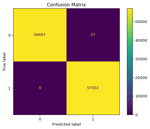
2. Train XGBoost Model
We initialize and train an XGBoost classifier using the balanced dataset.
Code
# Train XGBoost = XGBClassifier(eval_metric= 'logloss' , random_state= 42 , enable_categorical= False )# Evaluation = xgb.score(X_train, y_train)= xgb.score(X_test, y_test)print (f"Training Score: { train_score:.5f} " )print (f"Test Score: { test_score:.5f} " )# Predictions = xgb.predict(X_test)= xgb.predict_proba(X_test)[:, 1 ]= xgb.predict(X_full)= xgb.predict_proba(X_full)[:, 1 ]# Add predictions to original dataset = dataset.copy()'predictions' ] = xgb_preds_full'predictions_prob' ] = xgb_preds_full_prob# Confusion Matrix and Metrics = confusion_matrix(y_test, xgb_preds)'Confusion Matrix' )= pd.DataFrame({'Accuracy' : [round (accuracy_score(y_test, xgb_preds), 4 )],'Recall' : [round (recall_score(y_test, xgb_preds), 4 )],'Precision' : [round (precision_score(y_test, xgb_preds), 4 )],'F1 Score' : [round (f1_score(y_test, xgb_preds), 4 )]print (metrics)# ROC and AUC = roc_curve(y_test, xgb_preds_prob)= auc(fpr, tpr)= fpr, tpr= tpr, roc_auc= roc_auc).plot()'ROC Curve' )# Export "Data/output/xgboost_metrics.csv" , index= False )'fpr' : fpr, 'tpr' : tpr, 'thresh' : thresh}).to_csv("Data/output/xgboost_roc_curve_data.csv" , index= False )'AUC' : [roc_auc]}).to_csv("Data/output/xgboost_auc.csv" , index= False )"Data/output/xgboost_predictions.csv" , index= False )
Training Score: 0.99997
Test Score: 0.99967
   Accuracy  Recall  Precision  F1 Score
0    0.9997     1.0     0.9994    0.9997
3. Logistic Regression Model
In this section, we train a Logistic Regression model using the same balanced dataset and evaluate it using the same pipeline.
Train Logistic Regression Model
We train a logistic regression model for comparison using the same dataset.
Code
# Train Logistic Regression = LogisticRegression(max_iter= 1000 , random_state= 42 )# Evaluation = logreg.score(X_train, y_train)= logreg.score(X_test, y_test)print (f"Training Score: { train_score:.5f} " )print (f"Test Score: { test_score:.5f} " )# Predictions = logreg.predict(X_test)= logreg.predict_proba(X_test)[:, 1 ]= logreg.predict(X_full)= logreg.predict_proba(X_full)[:, 1 ]# Add predictions to original dataset = dataset.copy()'Data/output/logreg_predictions' ] = logreg_preds_full'Data/output/logreg_predictions_prob' ] = logreg_preds_full_prob# Confusion Matrix and Metrics = confusion_matrix(y_test, logreg_preds)'Confusion Matrix' )= pd.DataFrame({'Accuracy' : [round (accuracy_score(y_test, logreg_preds), 4 )],'Recall' : [round (recall_score(y_test, logreg_preds), 4 )],'Precision' : [round (precision_score(y_test, logreg_preds), 4 )],'F1 Score' : [round (f1_score(y_test, logreg_preds), 4 )]print (metrics)# ROC and AUC = roc_curve(y_test, logreg_preds_prob)= auc(fpr, tpr)= fpr, tpr= tpr, roc_auc= roc_auc).plot()'ROC Curve' )# Export "Data/output/logreg_metrics.csv" , index= False )'fpr' : fpr, 'tpr' : tpr, 'thresh' : thresh}).to_csv("Data/output/logreg_roc_curve_data.csv" , index= False )'AUC' : [roc_auc]}).to_csv("Data/output/logreg_auc.csv" , index= False )"Data/output/logreg_predictions.csv" , index= False )
Training Score: 0.94602
Test Score: 0.94641
   Accuracy  Recall  Precision  F1 Score
0    0.9464  0.9176      0.974    0.9449
4. Random Forest Classifier
Here we implement and evaluate a Random Forest classifier.
Make Predictions and Evaluate Model
Predictions are made on the test set and evaluated using accuracy, precision, recall, and F1-score.
Code
# Train Random Forest = RandomForestClassifier(n_estimators= 100 , random_state= 42 )# Evaluation = rf.score(X_train, y_train)= rf.score(X_test, y_test)print (f"Training Score: { train_score:.5f} " )print (f"Test Score: { test_score:.5f} " )# Predictions = rf.predict(X_test)= rf.predict_proba(X_test)[:, 1 ]= rf.predict(X_full)= rf.predict_proba(X_full)[:, 1 ]# Add predictions to original dataset = dataset.copy()'Data/output/rf_predictions' ] = rf_preds_full'Data/output/rf_predictions_prob' ] = rf_preds_full_prob# Confusion Matrix and Metrics = confusion_matrix(y_test, rf_preds)'Confusion Matrix' )= pd.DataFrame({'Accuracy' : [round (accuracy_score(y_test, rf_preds), 4 )],'Recall' : [round (recall_score(y_test, rf_preds), 4 )],'Precision' : [round (precision_score(y_test, rf_preds), 4 )],'F1 Score' : [round (f1_score(y_test, rf_preds), 4 )]print (metrics)# ROC and AUC = roc_curve(y_test, rf_preds_prob)= auc(fpr, tpr)= fpr, tpr= tpr, roc_auc= roc_auc).plot()'ROC Curve' )# Export "Data/output/rf_metrics.csv" , index= False )'fpr' : fpr, 'tpr' : tpr, 'thresh' : thresh}).to_csv("Data/output/rf_roc_curve_data.csv" , index= False )'AUC' : [roc_auc]}).to_csv("Data/output/rf_auc.csv" , index= False )"Data/output/rf_predictions.csv" , index= False )
Training Score: 1.00000
Test Score: 0.99991
   Accuracy  Recall  Precision  F1 Score
0    0.9999     1.0     0.9998    0.9999
5. LightGBM Classifier
We now train a LightGBM classifier and evaluate its performance similarly.
Train LightGBM Model
We train a LightGBM model with default parameters.
Code
# Train LightGBM = LGBMClassifier(random_state= 42 )# Evaluation = lgbm.score(X_train, y_train)= lgbm.score(X_test, y_test)print (f"Training Score: { train_score:.5f} " )print (f"Test Score: { test_score:.5f} " )# Predictions = lgbm.predict(X_test)= lgbm.predict_proba(X_test)[:, 1 ]= lgbm.predict(X_full)= lgbm.predict_proba(X_full)[:, 1 ]# Add predictions to original dataset = dataset.copy()'Data/output/lgbm_predictions' ] = lgbm_preds_full'Data/output/lgbm_predictions_prob' ] = lgbm_preds_full_prob# Confusion Matrix and Metrics = confusion_matrix(y_test, lgbm_preds)'Confusion Matrix' )= pd.DataFrame({'Accuracy' : [round (accuracy_score(y_test, lgbm_preds), 4 )],'Recall' : [round (recall_score(y_test, lgbm_preds), 4 )],'Precision' : [round (precision_score(y_test, lgbm_preds), 4 )],'F1 Score' : [round (f1_score(y_test, lgbm_preds), 4 )]print (metrics)# ROC and AUC = roc_curve(y_test, lgbm_preds_prob)= auc(fpr, tpr)= fpr, tpr= tpr, roc_auc= roc_auc).plot()'ROC Curve' )# Export "Data/output/lgbm_metrics.csv" , index= False )'fpr' : fpr, 'tpr' : tpr, 'thresh' : thresh}).to_csv("Data/output/lgbm_roc_curve_data.csv" , index= False )'AUC' : [roc_auc]}).to_csv("Data/output/lgbm_auc.csv" , index= False )"Data/output/lgbm_predictions.csv" , index= False )
[LightGBM] [Info] Number of positive: 227313, number of negative: 227591
[LightGBM] [Info] Auto-choosing col-wise multi-threading, the overhead of testing was 0.033456 seconds.
You can set `force_col_wise=true` to remove the overhead.
[LightGBM] [Info] Total Bins 7395
[LightGBM] [Info] Number of data points in the train set: 454904, number of used features: 29
[LightGBM] [Info] [binary:BoostFromScore]: pavg=0.499694 -> initscore=-0.001222
[LightGBM] [Info] Start training from score -0.001222
Training Score: 0.99935
Test Score: 0.99916
   Accuracy  Recall  Precision  F1 Score
0    0.9992     1.0     0.9984    0.9992
6. CatBoost Classifier
Finally, we train and evaluate a CatBoost classifier using the same pipeline.
Train CatBoost Model
This cell trains a CatBoost classifier, useful when handling categorical features.
Code
# Train CatBoost = CatBoostClassifier(verbose= 0 , random_state= 42 )# Evaluation = cat.score(X_train, y_train)= cat.score(X_test, y_test)print (f"Training Score: { train_score:.5f} " )print (f"Test Score: { test_score:.5f} " )# Predictions = cat.predict(X_test)= cat.predict_proba(X_test)[:, 1 ]= cat.predict(X_full)= cat.predict_proba(X_full)[:, 1 ]# Add predictions to original dataset = dataset.copy()'Data/output/cat_predictions' ] = cat_preds_full'Data/output/cat_predictions_prob' ] = cat_preds_full_prob# Confusion Matrix and Metrics = confusion_matrix(y_test, cat_preds)'Confusion Matrix' )= pd.DataFrame({'Accuracy' : [round (accuracy_score(y_test, cat_preds), 4 )],'Recall' : [round (recall_score(y_test, cat_preds), 4 )],'Precision' : [round (precision_score(y_test, cat_preds), 4 )],'F1 Score' : [round (f1_score(y_test, cat_preds), 4 )]print (metrics)# ROC and AUC = roc_curve(y_test, cat_preds_prob)= auc(fpr, tpr)= fpr, tpr= tpr, roc_auc= roc_auc).plot()'ROC Curve' )# Export "Data/output/cat_metrics.csv" , index= False )'fpr' : fpr, 'tpr' : tpr, 'thresh' : thresh}).to_csv("Data/output/cat_roc_curve_data.csv" , index= False )'AUC' : [roc_auc]}).to_csv("Data/output/cat_auc.csv" , index= False )"Data/output/cat_predictions.csv" , index= False )
Training Score: 0.99984
Test Score: 0.99960
   Accuracy  Recall  Precision  F1 Score
0    0.9996     1.0     0.9992    0.9996
7. Model Comparison Summary
We compare the evaluation metrics of all models side-by-side in a summary table.
8. Hyperparameter Tuning with GridSearchCV
We perform hyperparameter tuning on XGBoost using GridSearchCV to find the best parameters.
Train XGBoost Model
We initialize and train an XGBoost classifier using the balanced dataset.
Code
from sklearn.model_selection import GridSearchCV# Define parameter grid for XGBoost = {'max_depth' : [3 , 5 , 7 ],'learning_rate' : [0.01 , 0.1 ],'n_estimators' : [100 , 200 ],'subsample' : [0.8 , 1.0 ]= XGBClassifier(eval_metric= 'logloss' , random_state= 42 )= GridSearchCV(estimator= xgb_tune, param_grid= param_grid, cv= 3 , scoring= 'f1' , verbose= 1 , n_jobs=- 1 )print ("Best Parameters:" , grid_search.best_params_)= grid_search.best_estimator_# Evaluate tuned model = best_xgb.predict(X_test)= best_xgb.predict_proba(X_test)[:, 1 ]= pd.DataFrame({'Accuracy' : [accuracy_score(y_test, xgb_tuned_preds)],'Recall' : [recall_score(y_test, xgb_tuned_preds)],'Precision' : [precision_score(y_test, xgb_tuned_preds)],'F1 Score' : [f1_score(y_test, xgb_tuned_preds)]print (tuned_metrics)
Fitting 3 folds for each of 24 candidates, totalling 72 fits
Best Parameters: {'learning_rate': 0.1, 'max_depth': 7, 'n_estimators': 200, 'subsample': 0.8}
   Accuracy  Recall  Precision  F1 Score
0   0.99971     1.0   0.999421  0.999711
9. Ensemble Model (Voting Classifier)
We combine XGBoost, Random Forest, and Logistic Regression into an ensemble Voting Classifier to leverage their strengths.
Train XGBoost Model
We initialize and train an XGBoost classifier using the balanced dataset.
Code
from sklearn.ensemble import VotingClassifier# Define base models = XGBClassifier(eval_metric= 'logloss' , random_state= 42 )= RandomForestClassifier(n_estimators= 100 , random_state= 42 )= LogisticRegression(max_iter= 1000 , random_state= 42 )# Create ensemble model = VotingClassifier(estimators= ['xgb' , xgb_base),'rf' , rf_base),'lr' , logreg_base)= 'soft' )= voting_clf.predict(X_test)= voting_clf.predict_proba(X_test)[:, 1 ]# Evaluate ensemble = pd.DataFrame({'Accuracy' : [accuracy_score(y_test, ensemble_preds)],'Recall' : [recall_score(y_test, ensemble_preds)],'Precision' : [precision_score(y_test, ensemble_preds)],'F1 Score' : [f1_score(y_test, ensemble_preds)]print (ensemble_metrics)# Save to CSV "Data/output/ensemble_metrics.csv" , index= False )
   Accuracy  Recall  Precision  F1 Score
0   0.99978     1.0   0.999562  0.999781
10. Stacking Ensemble
We use StackingClassifier to combine base models and a meta-model for improved performance.
Train XGBoost Model
We initialize and train an XGBoost classifier using the balanced dataset.
Code
from sklearn.ensemble import StackingClassifier# Define base learners and meta-learner = ['rf' , RandomForestClassifier(n_estimators= 100 , random_state= 42 )),'lr' , LogisticRegression(max_iter= 1000 , random_state= 42 )),'xgb' , XGBClassifier(eval_metric= 'logloss' , random_state= 42 ))= StackingClassifier(estimators= estimators, final_estimator= LogisticRegression(), cv= 3 )= stack_model.predict(X_test)= stack_model.predict_proba(X_test)[:, 1 ]= pd.DataFrame({'Accuracy' : [accuracy_score(y_test, stack_preds)],'Recall' : [recall_score(y_test, stack_preds)],'Precision' : [precision_score(y_test, stack_preds)],'F1 Score' : [f1_score(y_test, stack_preds)]print (stack_metrics)"Data/output/stacking_metrics.csv" , index= False )
   Accuracy  Recall  Precision  F1 Score
0  0.999877     1.0   0.999754  0.999877
11. AutoML-Style Comparison Table
Aggregate metrics from all models including tuned and ensemble methods for a final comparison.
12. Deployment-Ready Script Generator
Export the best model and required transformers for future inference (e.g. in Flask or Streamlit).